The Data

The data for the competition can be downloaded here: https://www.kaggle.com/c/talkingdata-mobile-user-demographics/data .

I have downloaded and read each file into R, giving each data.frame the same name as the file. Below are the first 3 records of each file.

head(app_events, 3)

event_id	app_id	is_installed	is_active
1924946	3.489720e+18	1	1
19620	7.723979e+18	1	1
53629	7.723979e+18	1	1

head(app_labels, 3)

app_id	label_id
-2.600988e+18	2
-2.600988e+18	4
4.214070e+18	5

head(events, 3)

event_id	device_id	timestamp	longitude	latitude	region	date	hour	time
1924946	-7.013555e+18	2016-05-06 07:39:53	109.46	21.89	NA	2016-05-06	7	morning
19620	8.427965e+18	2016-05-07 17:38:53	117.35	25.34	NA	2016-05-07	17	midday
53629	-6.506152e+18	2016-05-03 18:55:04	0.00	0.00	NA	2016-05-03	18	evening

head(gender_age_train, 3)

device_id	gender	age	group
8.427965e+18	F	23	F23-
-3.293695e+18	M	40	M39+
7.104535e+18	M	25	M23-26

head(phone_brand_device_model, 3) # Chinese characters displayed in UTF-8 codes

device_id	phone_brand	device_model
8.427965e+18	vivo	X5M
1.186608e+18		2
1.186608e+18

The number of records in each data.frame can be seen in the table below.

Table	Records
app_events	12,732,996
app_labels	459,943
events	3,252,950
gender_age_train	74,645
phone_brand_device_model	187,245

And below is the data schema provided on the Kaggle site.

Tidy Data

For our purpose, it is more convenient to look at the data in one nice “tidy” table. I have joined the tables and created some new columns that help make sense of the data. You can see the data by clicking on “Data Table” in the banner above. Below is a data dictionary.

Fields	Description
event_id	Unique mobile event identifier. The primary key for this table.
device_id	The mobile device identifier. Demographics are associated with this number.
longitude; latitude	Geolocation
region	Feature generated from the data. Most events in china take place in three cities: Beijing, Chengdu, Hong Kong, and Shanghai.
date; hour; time	Time
gender; age	Demographics
phone_brand; device_model	Mobile device brand information.
apps	Feature generated from the data. The number of active apps during the event.
Custom; Education; etc.	These columns are also features generated from the data. These are categories of apps that are active during the event. A value of 1 means that at least 1 app from this category is active. See the file generalizeCategories.R in the GitHub repository for the R code that generated these features.

Note: The Chinese characters for the phone brand and device model are rendered as their UTF-8 code or sometimes not at all.

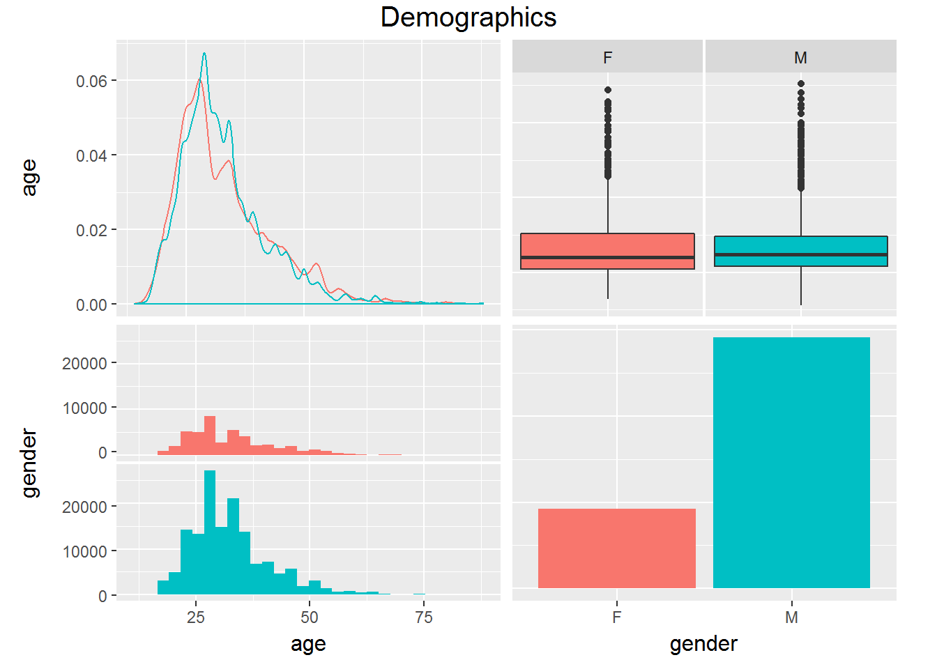
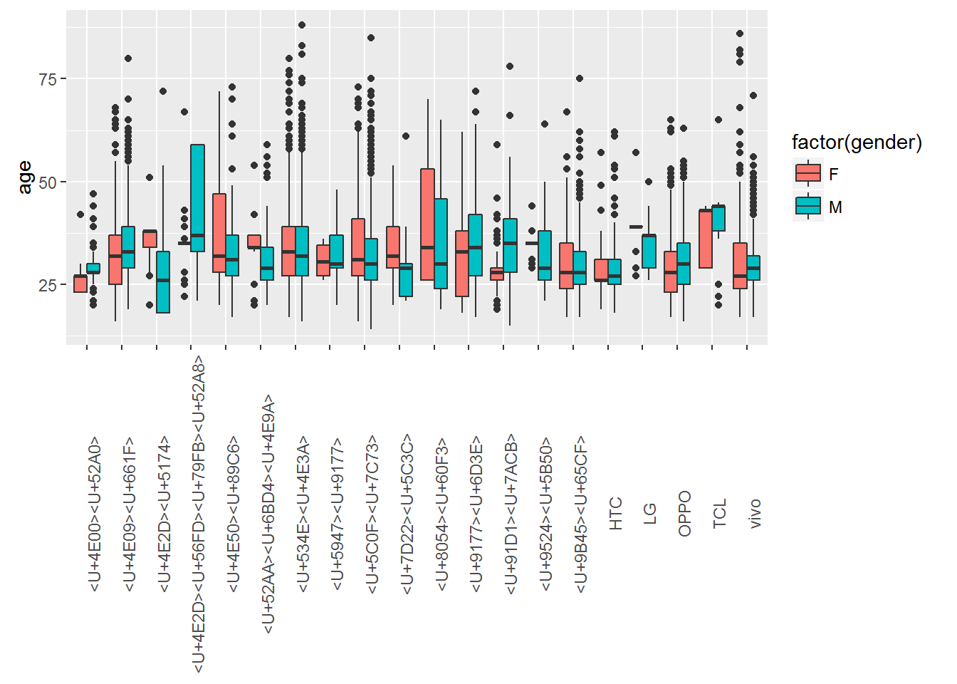
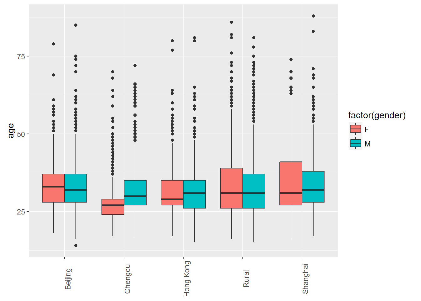
Data Exploration

The tidy data set can be visualized using the TalkingData Explorer found here: https://natebyers.shinyapps.io/TalkingData_Explorer/ .

Below are plots that vizualize the distribution of gender and age.

Prediction

Random forest model for predicting gender.

library(caret)
for(i in names(full_data)){
  if(class(full_data[[i]]) == "character"){
    full_data[[i]] <- as.factor(full_data[[i]])
  }
}

gender_subset <- full_data %>%
  arrange(gender) %>%
  sample_n(2000) %>%
  select(gender, region, hour, phone_brand, Games, Education, Finance)

ctrl <- trainControl(method="repeatedcv", number=2, repeats=1, 
                     selectionFunction = "oneSE")
in_train <- createDataPartition(gender_subset$gender, p=.80, list=FALSE)

rf <- train(gender ~ ., data = gender_subset, method = "rf",
            metric = "Kappa", trControl = ctrl, subset = in_train)

test <- gender_subset[-in_train,]
test$pred <- predict(rf, test, "raw")
confusionMatrix(test$pred, test$gender)

## Confusion Matrix and Statistics
## 
##           Reference
## Prediction   F   M
##          F  10  19
##          M  90 280
##                                         
##                Accuracy : 0.7268        
##                  95% CI : (0.6803, 0.77)
##     No Information Rate : 0.7494        
##     P-Value [Acc > NIR] : 0.8634        
##                                         
##                   Kappa : 0.0477        
##  Mcnemar's Test P-Value : 2.017e-11     
##                                         
##             Sensitivity : 0.10000       
##             Specificity : 0.93645       
##          Pos Pred Value : 0.34483       
##          Neg Pred Value : 0.75676       
##              Prevalence : 0.25063       
##          Detection Rate : 0.02506       
##    Detection Prevalence : 0.07268       
##       Balanced Accuracy : 0.51823       
##                                         
##        'Positive' Class : F             
## 

prd <- data.frame(region = "Hong Kong", hour = 12, phone_brand = "vivo",
                  Games = 1, Education = 1, Finance = 0)
predict(rf, prd)

## [1] M
## Levels: F M

Linear model for predicting age.

age_subset <- full_data %>%
  arrange(age) %>%
  sample_n(2000)

split<-createDataPartition(age_subset$age, p = 0.6, list = FALSE)

dev<-age_subset[split,] %>%
  select(age, region, hour, phone_brand, Games, Education,
         Finance)

val<-age_subset[-split,] %>%
  select(age, region, hour, phone_brand, Games, Education,
         Finance)

ctrl<-trainControl(method = "cv", number = 2)

lm<-train(age~., data = dev, method = "lm", trControl = ctrl)

lm

## Linear Regression 
## 
## 1202 samples
##    6 predictor
## 
## No pre-processing
## Resampling: Cross-Validated (2 fold) 
## Summary of sample sizes: 602, 600 
## Resampling results:
## 
##   RMSE      Rsquared  
##   9.129228  0.03066149
## 
## 

predict(lm, prd)

##        1 
## 27.83763

Application

The models can be used to make a prediction of the users gender and age. Below is an application that gives an estimated age and gender based on the user inputs.